Chemical Reactions, Flux and Transport

Mechanica supports modeling and simulation of fluids using Dissipative Particle Dynamics (DPD), where each particle represents a ‘parcel’ of a real fluid. A single DPD particle typically represents anywhere from a cubic micron to a cubic mm, or about \(3.3 \times 10^{10}\) to \(3.3 \times 10^{19}\) water molecules. DPD particle interactions are implemented in Mechanica using the dpd potential.

Building on DPD capabilities, Mechanica also supports attaching diffusive chemical solutes to DPD-like particles using Transport Dissipative Particle Dynamics (tDPD), where each tDPD particle represents a parcel of bulk fluid with a set of chemical solutes at each particle. Chemical solutes in Mechanica are referred to as species. In tDPD, a particle represents a parcel of the bulk medium, or the ‘solvent’, and each tDPD particle carries along, or advects, attached solutes. Solutes can diffuse between nearby tDPD particles, and can be created and destroyed through various reaction processes.

In general, the time evolution of a chemical species attached to the \(i\mathrm{th}\) particle \(S_i\) is given as:

\[\frac{dS_i}{dt} = \sum_{i \neq j} Q^T_{ij} +Q^R_i,\]

where the rate of change of the chemical species attached to a particle is equal to the sum of the transport flux \(Q^T\) and local reactions \(Q^R_i\).

Species can be added to a particle type by simply adding a species attribute to a particle type class definition and assigning a list of names, each of which names a species. Mechancia automatically instantiates each corresponding particle of the particle type with a species of each specified name.

import mechanica as mx

class AType(mx.ParticleType):
    species = ['S1', 'S2', 'S3']

An instance of a particle type with attached chemical species has a vector of chemical species attached to it, which is accessible via the attribute species. Likewise each particle with attached chemical species has a state vector with a value assigned to each attached species, which is also accessible via the attribute species.

A = AType.get()
print(A.species)  # prints SpeciesList(['S1', 'S2', 'S3'])
a = A()
print(a.species)  # prints StateVector([S1:0, S2:0, S3:0])

SpeciesList (MxSpeciesList in C++) is a special list of SBML species definitions. SpeciesList can also be created with additional information about the species by instantiating with instances of the Mechanica class Species (MxSpecies in C++).

The state vector of type StateVector (MxStateVector in C++) attached to each particle is array-like but, in addition to the numerical values of the species, also contains metadata of the species definitions. The concentration of a particular species in a particle can be accessed by index or name.

print(a.species[0])  # prints 0.0
a.species.S1 = 1
print(a.species[0])  # prints 1.0
a.species[0] = 5
print(a.species.S1)  # prints 5.0

Working with Species

By default, Mechanica creates Species instances that are floating species, or species with a concentration that varies in time, and that participate in reaction and flux processes. However, Mechanica also supports other kinds of species such as boundary species, as well as additional information about the species like its initial values.

The Mechanica Species class is essentially a wrap around the libSBML Species class, but provides some conveniences in generated languages. For example, in Python Mechanica uses convential Python snake_case sytax, and all SBML Species properties are avialable via simple properties on a Mechanica Species object. Many SBML concepts such as initial_amount, constant, etc. are optional features in Mechanica that may or may not be set. For example, to set an initial concentration on a Species instance s,

s.initial_concentration = 5.0

Such operations internally update the libSBML Species instance contained within the Mechanica Species instance, and Mechanica will use the information accordingly. In the case of initial_concentration, the value determines the initial concentration of created particles when the Species belongs to a particular particle type. Likewise, setting the attribute constant of a Species belonging to a particle type to True makes all created particles of that type maintaing a constant concentration (and for a particular particle when the Species instance belongs to a particle),

# Make all particles of type 'a' have constant concentration...
a.species.S1.constant = True
# ... except let this one vary
a_part = a()
a_part.species.species.S1.constant = False

In the simplest case, a Mechanica Species instance can be created by constructing with only the name of the species.

s = mx.Species("S1")

A species can be made a boundary species (i.e., one that acts like a boundary condition) by adding "$" in the argument.

bs = mx.Species("$S2")
print(bs.id)        # prints 'S2'
print(bs.boundary)  # prints True

The Species constructor also supports specifying initial values, which can be made using an equality statement.

ia = mx.Species("S3 = 1.2345")
print(ia.id)              # prints 'S3'
print(ia.initial_amount)  # prints 1.2345

When constructing a SpeciesList with Species instances, an empty SpeciesList instance is first created, to which Species instances are appended using the SpeciesList method insert.

s_list = mx.SpeciesList()
s_list.insert(s)
s_list.insert(ia)
print(s_list)  # prints SpeciesList(['S1', 'S3'])

Each species in a SpeciesList instance can be accessed using the SpeciesList method item.

print(s_list.item("S1").id)  # prints 'S1'

Spatial Transport

Recall that the DPD-like particles in Mechanica (and in general) represent a parcel of fluid. Mechanica tDPD modeling provides a natural way of modeling advection by the mere motion of particles carrying species. Furthermore, Mechanica also provides the ability to model the tendency of dissolved chemical solutes in each parcel of fluid to diffuse to nearby locations, which results in mixing or mass transport without directed bulk motion of the solvent. Modeling convection in Mechanica is then the combination of transporting species along with tDPD particles (i.e., advection) and between tDPD particles (i.e., diffusion).

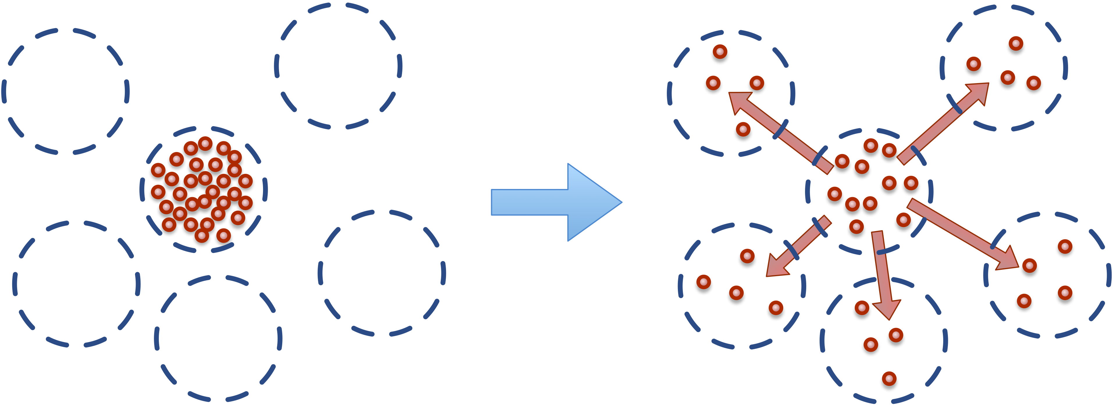
Fig. 6 Dissolved solutes have a natural tendency to diffuse to nearby locations.

A flux describes the transport of species between particles. Fluxes are similar to pair-wise forces between particles, in that a flux transports a particular species between nearby particles of particular particle types. A flux that implements a Fickian diffusion process of chemical species located at particles can be created with the static method flux on a top-level class Fluxes (MxFluxes in C++). Mechanica implements a diffusion process of chemical species located at particles using the basic passive (Fickian) flux type, with flux. Fickian flux implements a diffusive transport of species concentration \(S\) located on a pair of nearby objects \(a\) and \(b\) with the analogous reaction:

\[\begin{split}\begin{align*} a.S \leftrightarrow b.S &; k \left(1 - \frac{r}{r_{cutoff}} \right)\left(a.S - b.S\right) \\ a.S \rightarrow 0 &; \frac{d}{2} a.S \\ b.S \rightarrow 0 &; \frac{d}{2} b.S, \end{align*}\end{split}\]

Here \(a.S\) is a chemical species located at object \(a\), and likewise for \(b\), \(k\) is the flux constant, \(r\) is the distance between the two objects, \(r_{cutoff}\) is the global cutoff distance, and \(d\) is the optional decay term.

Fickian diffusion can be implemented on the basis of species and pair of particle types.

class AType(mx.ParticleType)
    species = ['S1']

class BType(mx.ParticleType)
    species = ['S1', 'S2']

A = AType.get(); B = BType.get()

mx.Fluxes.flux(A, A, 'S1', 5.0)

Likewise, decay can also be assigned as an optional fourth argument.

mx.Fluxes.flux(B, B, 'S2', 7.5, 0.005)

Production and Consumption

Mechanica supports modeling active pumping for applications like membrane ion pumps, or other forms of active transport with the methods secrete and uptake, which are also defined on Fluxes.

The secrete flux implements the reaction:

\[\begin{split}\begin{align*} a.S \rightarrow b.S &; k \left(1 - \frac{r}{r_{cutoff}} \right)\left(a.S - a.S_{target} \right) \\ a.S \rightarrow 0 &; \frac{d}{2} a.S \\ b.S \rightarrow 0 &; \frac{d}{2} b.S \end{align*}\end{split}\]

The uptake flux implements the reaction:

\[\begin{split}\begin{align*} a.S \rightarrow b.S &; k \left(1 - \frac{r}{r_{cutoff}}\right)\left(b.S - b.S_{target} \right)\left(a.S\right) \\ a.S \rightarrow 0 &; \frac{d}{2} a.S \\ b.S \rightarrow 0 &; \frac{d}{2} b.S \end{align*}\end{split}\]

Here \(S_{target}\) is a target concentration, and all other symbols are as previously defined. Note that changes in sign due to the difference of the present and target concentrations are permissible. Both methods require the same arguments as flux and a fourth argument defining the target concentration.

mx.Fluxes.secrete(A, B, 'S1', 10.0, 1.0)

An optional decay term can also be included for both methods as a fifth argument.

mx.Fluxes.uptake(B, A, 'S1', 10.0, 1.0, 0.001)

Species can also be secreted directly from a particle to its surroundings. A species attached to a particle has a method secrete that takes the argument of an amount to be released over the current time step.

a = A()
a.species.S1.secrete(10.0)

The neighborhood to which a species is secreted can be explicitly defined by distance from a particle using the keyword argument distance.

b = B()
b.species.S1.secrete(5.0, distance=1.0)

The neighborhood can also be defined in terms of particles by passing a ParticleList instance to the keyword argument to.

b.species.S1.secrete(5.0, to=b.neighbors())