Quickstart

Python Quickstart

This example will create a complete simulation of a set of argon atoms in Python. First we simply import Mechanica, and we will also use Numpy to create initial conditions:

import mechanica as mx
import numpy as np

We’ll start by defining a variable that defines the size of the simulation domain. Among many other ways to configure a simulation, we can specify the size of the universe in a simulation using a list:

# dimensions of universe
dim = [10., 10., 10.]

The first thing we must always do before we create any Mechanica simulation object is initialize Mechanica. This essentially sets up the simulation environment, and gives us a place to create our model.

mx.init(dim=dim)

A Mechanica particle type acts like a factory that creates particles according to its definition. Mechanica provides more than one way to create a custom particle type. However, the recommend method of designing a new particle type is to create a subclass of the Mechanica base particle type (ParticleType in Python). The Mechanica particle type (and corresponding particles) contains a number of customizable attributes such as radius and mass.

# create a particle type
class ArgonType(mx.ParticleType):
    mass = 39.4

A new, derived particle type must be registered with Mechanica before we can use it to create particles. We can use the same class method to register and get our new particle type, and no matter where we might be in a script, we can use the same class method to always get the instance of our particle type that Mechanica is also using to simulate our model.

# Register and get the particle type; registration always only occurs once
Argon = ArgonType.get()

Note

Particle types are not automatically registered with Mechanica in Python when simply instantiated. Mechanica follows this paradigm to facilitate model archiving and sharing, as well as basic model-specific operations that do not require simulation functionality.

Particles can interact via Potentials (Potential in Python). Mechanica provides a variety of built-in potentials, as well as the ability to create custom interactions. For now, we will use the built-in Lennard-Jones 12-6 potential. All we have to do is create an instance of a potential and bind it to objects that interact according to our model. To create a Lennard-Jones 12-6 potential,

# create a potential representing a 12-6 Lennard-Jones potential
pot = m.Potential.lennard_jones_12_6(0.275, 3.0, 9.5075e-06, 6.1545e-03, 1.0e-3)

The total force on any object such as a particle is simply the sum of all forces that act on that object. To make our potential describe an interaction force between all particles of our new particle type, we bind our potential to our new type:

# bind the potential with the *TYPES* of the particles
mx.bind.types(pot, Argon, Argon)

Note

Argon is passed as both the second and third arguments of bind.types because we are here describing an interaction between particles of two types. We could do the same to describe an interaction between Argon particles and particles of some other type that we might create.

To fill our simulation domain with particles at uniformly distributed random initial positions, we can use a numpy random function to generate an array of positions:

# uniform random cube
positions = np.random.uniform(low=0, high=10, size=(10000, 3))

We then simply create a new particle at each of our positions using our new particle type. We can create particles of our new particle type by using it like a function:

for pos in positions:
    # calling the particle constructor implicitly adds
    # the particle to the universe
    Argon(pos)

Now all that’s left is to run our simulation. The Mechanica Python module has two methods to run a simulation: run and irun. The run method runs the simulation, and (if no final time is passed as argument) continues until the window is closed, or some stop condition. If running Mechanica from IPython, the irun method starts the simulation but leaves the console open for further input.

# run the simulator interactive
m.Simulator.run()

Putting it all together looks something like the following. The complete script can also be downloaded here:

Download: this example script:

import mechanica as mx
import numpy as np

# dimensions of universe
dim = [10., 10., 10.]

# new simulator
mx.init(dim=dim)

# create a potential representing a 12-6 Lennard-Jones potential
pot = mx.Potential.lennard_jones_12_6(0.275, 3.0, 9.5075e-06, 6.1545e-03, 1.0e-3)


# create a particle type
class ArgonType(mx.ParticleType):
    radius = 0.1
    mass = 39.4


# Register and get the particle type; registration always only occurs once
Argon = ArgonType.get()

# bind the potential with the *TYPES* of the particles
mx.bind.types(pot, Argon, Argon)

# uniform random cube
positions = np.random.uniform(low=0, high=10, size=(10000, 3))

for pos in positions:
    # calling the particle constructor implicitly adds
    # the particle to the universe
    Argon(pos)

# run the simulator interactive
mx.run()

C++ Quickstart

This example will create a complete simulation of a set of argon atoms in C++ that can be compiled into an executable program. First, we create a basic skeleton of an entry point and simulation function.

int quickstart() {
    return 0;
}

int main (int argc, char** argv) {
    return quickstart();
}

Among many other ways to configure a simulation, we can specify the size of the universe in a simulation using a MxSimulator_Config object defined in MxSimulator.h. We add at the top of our script:

#include <MxSimulator.h>

Then we begin our quickstart function:

MxSimulator_Config config;
config.universeConfig.dim = {10., 10., 10.};

The first thing we must always do before we create any Mechanica simulation object is initialize Mechanica. This essentially sets up the simulation environment, and gives us a place to create our model. We add to the end of our quickstart function,

MxSimulator_initC(config);

A Mechanica particle type acts like a factory that creates particles according to its definition. Mechanica provides more than one way to create a custom particle type. However, the recommend method of designing a new particle type is to create a subclass of the Mechanica base particle type (MxParticleType in C++). The Mechanica particle type (and corresponding particles) contains a number of customizable attributes such as radius and mass, and is defined in MxParticle.h. We add at the top of of script,

#include <MxParticle.h>

Then we add before our quickstart function the definition of our new particle type:

struct ArgonType : MxParticleType {
    ArgonType() : MxParticleType(true) {
        radius = 0.1;
        mass = 39.4;
        registerType();
    }
};

A new, derived particle type must be registered with Mechanica before we can use it to create particles. We can use the same class method to register and get our new particle type, and no matter where we might be in a script, we can use the same class method to always get the instance of our particle type that Mechanica is also using to simulate our model. We add to the end of our quickstart function,

ArgonType *Argon = new ArgonType();
Argon = (ArgonType*)Argon->get();

Note

Particle types are not automatically registered with Mechanica in C++ when instantiated with a true argument. Mechanica permits this functionality to facilitate model archiving and sharing, as well as basic model-specific operations that do not require simulation functionality.

Particles can interact via Potentials (MxPotential in C++). Mechanica provides a variety of built-in potentials, as well as the ability to create custom interactions. For now, we will use the built-in Lennard-Jones 12-6 potential. All we have to do is create an instance of a potential using definitions in MxPotential.h and bind it to objects that interact according to our model. To create a Lennard-Jones 12-6 potential, we add at the top of our script,

#include <MxPotential.h>

We add to the end of our quickstart function,

MxPotential *pot = MxPotential::lennard_jones_12_6(0.275, 3.0, 9.5075e-06 , 6.1545e-03 , new double(1.0e-3));

The total force on any object such as a particle is simply the sum of all forces that act on that object. To make our potential describe an interaction force between all particles of our new particle type, we bind our potential to our new type using definitions in MxBind.hpp. We add at the top of our script

#include <MxBind.hpp>

We add to the end of our quickstart function,

MxBind::types(pot, Argon, Argon);

Note

Argon is passed as both the second and third arguments of bind.types because we are here describing an interaction between particles of two types. We could do the same to describe an interaction between Argon particles and particles of some other type that we might create.

To fill our simulation domain with particles at uniformly distributed random initial positions, we can use a Mechanica function defined in MxUtil.h to generate an array of positions in a unit cube centered at the origin. We add at the top of our script

#include <MxUtil.h>

We add to the end of our quickstart function,

std::vector<MxVector3f> positions = MxRandomPoints(MxPointsType::SolidCube, 10000);

We then simply create a new particle at each of our positions using our new particle type. We can create particles of our new particle type by using it like a function. We add to the end of our quickstart function,

for(auto &p : positions) {
    MxVector3f *partPos = new MxVector3f((p + MxVector3f(0.5)) * 10.0);
    (*Argon)(partPos);
}

Now all that’s left is to run our simulation. The Mechanica MxSimulator has a method run that runs the simulation, and (if a negative number is passed) continues until the window is closed, or some stop condition. We add to the end of our quickstart function,

MxSimulator *sim = MxSimulator::get();
sim->run(-1.0);

Putting it all together looks something like the following:

#include <MxSimulator.h>
#include <MxParticle.h>
#include <MxPotential.h>
#include <MxBind.hpp>
#include <MxUtil.h>

struct ArgonType : MxParticleType {
    ArgonType() : MxParticleType(true) {
        radius = 0.1;
        mass = 39.4;
        registerType();
    }
};

int quickstart() {
    MxSimulator_Config config;
    config.universeConfig.dim = {10., 10., 10.};
    MxSimulator_initC(config);

    ArgonType *Argon = new ArgonType();
    Argon = (ArgonType*)Argon->get();

    MxPotential *pot = MxPotential::lennard_jones_12_6(0.275, 3.0, 9.5075e-06 , 6.1545e-03 , new double(1.0e-3));
    MxBind::types(pot, Argon, Argon);

    std::vector<MxVector3f> positions = MxRandomPoints(MxPointsType::SolidCube, 10000);

    for(auto &p : positions) {
        MxVector3f *partPos = new MxVector3f((p + MxVector3f(0.5)) * 10.0);
        (*Argon)(partPos);
    }

    MxSimulator *sim = MxSimulator::get();
    sim->run(-1.0);

    return 0;
}

int main (int argc, char** argv) {
    return quickstart();
}

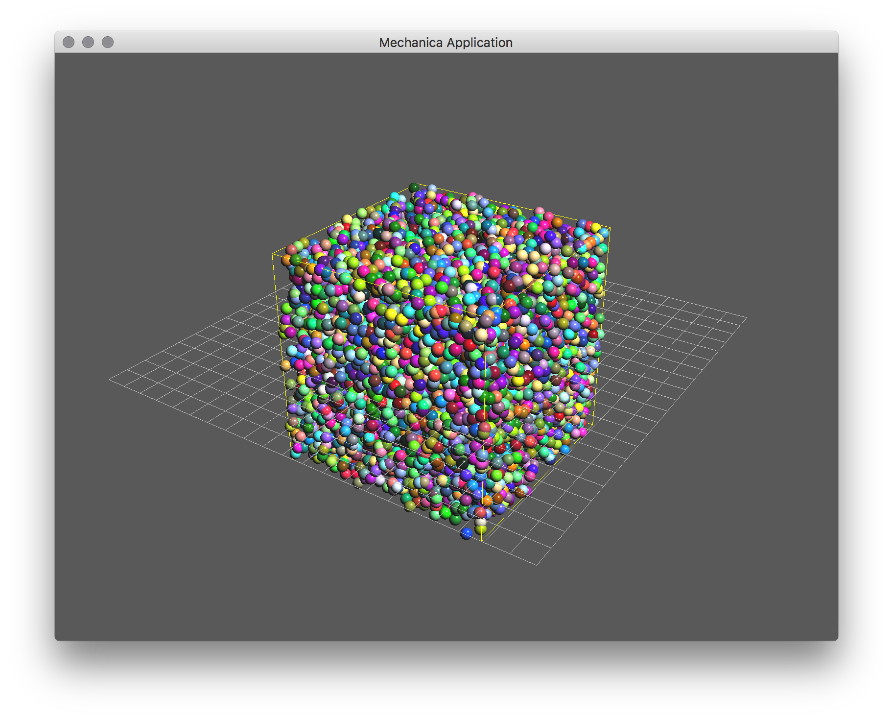
Fig. 3 A basic argon simulation