Potentials
One of the main goals of Mechanica is to enable users to rapidly develop and explore empirical or phenomenological models of active and biological matter in the 100nm to multiple cm range. Supporting modeling and simulation in these ranges requires a good deal of flexibility to create and calibrate potential functions to model material rheology and particle interactions.
Mechanica provides a wide range of potentials in the Potential class
(MxPotential in C++). Any of the built-in potential functions
can be created as objects in a simulation using a static method on the
Potential class, which can be bound to pairs and
groups of particles to implement models of interactions.
Creating, Plotting and Exploring Potentials
Potential objects are created simply by calling one of the
static methods on the Potential class. In Python, Potential
objects conveniently have a plot method that displays a matplotlib
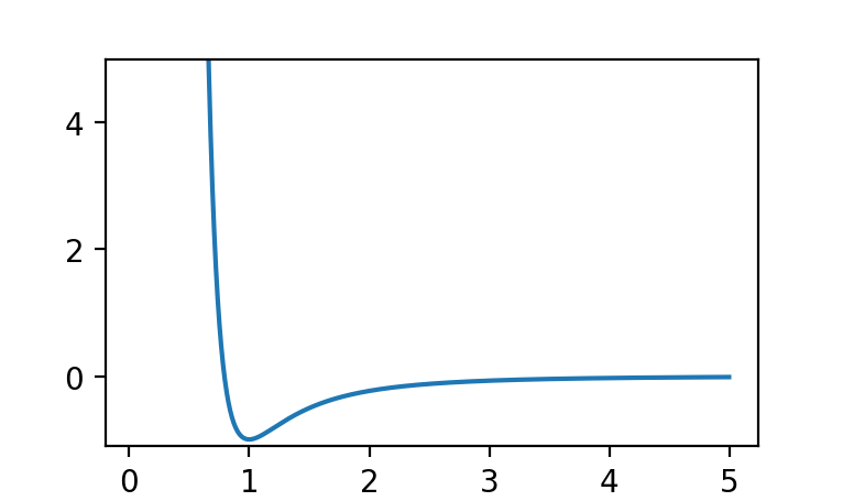
plot. For example, while working with the built-in
Generalized Lennard-Jones potential,
import mechanica as mx
pot = mx.Potential.glj(10)
pot.plot()
results in
A Potential instance can also be created by adding two existing
instances. Such operations can be arbitrarily performed to construct complicated
potentials consisting of multiple constituent potentials,
pot_charged = mx.Potential.coulomb(q=1)
pot_fluid = mx.Potential.dpd(alpha=0.3, gamma=1, sigma=1, cutoff=0.6)
pot_charged_fluid = pot_charged + pot_fluid
Note
Changes to constituent potentials during simulation are reflected in potentials that have been constructed from them using summation operations.
Mechanica also supports creating custom potentials with the Potential method
custom. A custom potential requires the domain of the potential and, at minimum,
a function that takes a float as argument and returns the value of the potential at the
argument value. Mechanica constructs an interpolation of a potential function using
functions that return the value of the potential, its first derivative, and its
sixth derivative. When a function is not provided for either derivative, the derivative
is approximated using finite difference,
pot_custom = mx.Potential.custom(min=0.0, max=2.0,
                                 f=lambda r: (r-1.0) ** 6.0,            # Potential function
                                 fp=lambda r: 6.0 * (r-1.0) ** 5.0,     # First derivative
                                 f6p=lambda r: 720.0)                   # Sixth derivative
Potentials for angle and
dihedral bonds by passing Potential.Flags.angle.value
and Potential.Flags.dihedral.value, respectively, to the keyword argument flags. In
both cases, the cosine of the angle of an angle or dihedral bond is passed as argument to
the potential function,
pot_angle = mx.Potential.custom(min=-0.999, max=0.999,
                                f=lambda r: cos(2.0 * acos(r)),
                                flags=mx.Potential.Flags.angle.value)
Note
The cosine of angles is used when evaluating angle and dihedral bonds to improve
computational performance, but presents challenges to creating custom potentials in
that analytic expressions for derivatives of the potential function can be excessively
tedious to derive and implement. This issue motivates providing built-in support
for approximating derivatives using finite difference. However, providing functions
for the first and sixth derivative of a potential function is recommended whenever possible,
as is examining the quality of the generated interpolation of a potential function before
using it in a simulation using plot.
Built-in Potentials
Presently, the following built-in potential functions are supported, with corresponding constructor method. For details on the parameters of each function, refer to the Mechanica API Reference.
12-6 Lennard-Jones: Potential.lennard_jones_12_6
12-6 Lennard-Jones with shifted Coulomb: Potential.lennard_jones_12_6_coulomb
Coulomb: Potential.coulomb
Coulomb reciprocal potential: Potential.coulombR
Dissipative particle dynamics: Potential.dpd
Ewald (real-space): Potential.ewald
Generalized Lennard-Jones: Potential.glj
Harmonic: Potential.harmonic
Harmonic angle: Potential.harmonic_angle
Harmonic dihedral: Potential.harmonic_dihedral
Cosine dihedral: Potential.cosine_dihedral
Linear: Potential.linear
Morse: Potential.morse
Overlapping sphere: Potential.overlapping_sphere
Power: Potential.power
Soft sphere: Potential.soft_sphere
Well: Potential.well